Goodness of Fit and Contingency chi-squared tests
Emma Rand

Introduction
Aims
To explain how to analyse data that are counts falling into mutually exclusive categories using two types of chi-squared test and the difference between these two tests.
Learning Outcomes
By actively following the lecture and practical and carrying out the independent study the successful student will be able to:
- recognise when to use chi-squared Goodness of Fit and Contingency tests (MLO 2)
- be able to carry out, interpret and report scientifically both types in R (MLO 3 and 4)
Philosophy
Workshops are not a test. It is expected that you often don’t know how to start, make a lot of mistakes and need help. Do not be put off and don’t let what you can not do interfere with what you can do. You will benefit from collaborating with others and/or discussing your results.
The lectures and the workshops are closely integrated and it is expected that you are familar with the lecture content before the workshop. You need not understand every detail as the workshop should build and consolidate your understanding. You may wish to refer to the slides as you work through the workshop schedule.
Getting started
 Start RStudio from the Start menu.
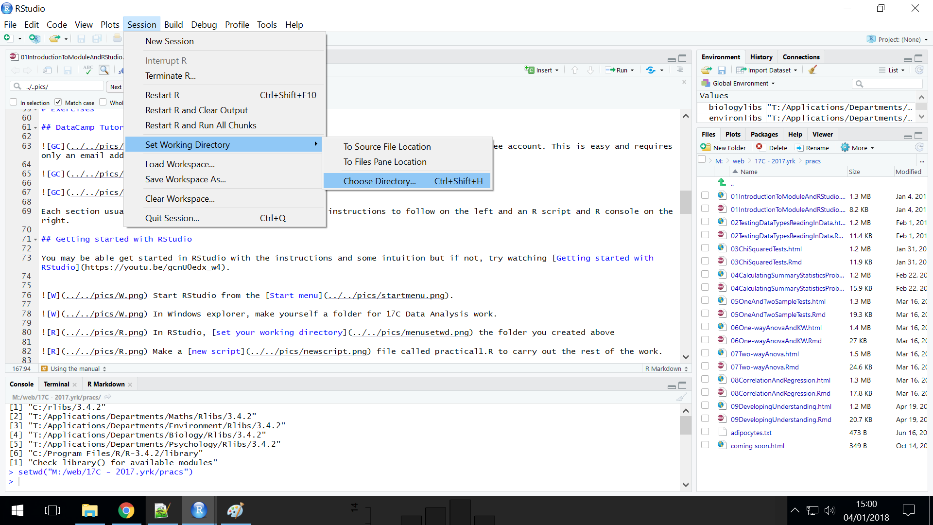
 In RStudio, set your working directory to the folder you created last week for your 17C Data Analysis work.
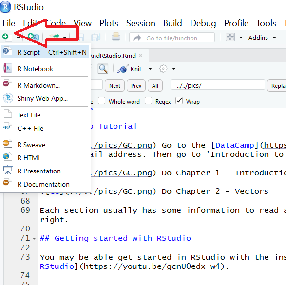
Make a new script file called practical3.R to carry out the rest of the work.
Exercises
Inductions
In a local maternity hospital, the total numbers of births induced on each day of the week over a six week period were recorded a
| Day | No.inductions |
|---|---|
| Monday | 43 |
| Tuesday | 36 |
| Wednesday | 35 |
| Thursday | 38 |
| Friday | 48 |
| Saturday | 26 |
| Sunday | 24 |
| Total | 250 |
Inductions - coding the \({\chi}^2\)
We can use a chi-squared test to ascertain whether there is a pattern in these data that might suggest that surgeons are more reluctant to perform inductions on some days than on others.
Make a vector obs that holds the number of inductions on each day.
Examine the ‘structure’ of the obs object using str()
 What is your null hypothesis and what type of test is required?
We can carry out a Goodness of Fit chi-squared test on these data by coding the how the test works ourselves. If the null hypothesis is true, 1/7th of inductions would be expected to occur each day i.e., 1/7th of 250
Assign the total number of inductions to a variable called totalinductions
Now calculate the expected values:
# the expected values
# note that R mulitples every element in the c() by totalinductions
exp <- c(1/7, 1/7, 1/7, 1/7, 1/7, 1/7, 1/7) * totalinductions
The formula for chi-squared is: \({\chi}^2 = \Sigma \frac{(O - E)^2}{E}\)
We can write this in R using:
We have \({\chi}^2 =\) 12.36
The degrees of freedom for a Goodness of fit chi-squared test are the number of categories minus one.
Calculate and assign the d.f. to a variable called df
The p value can be calculated with:
## [1] 0.05440298 What do you conclude about the pattern of birth inductions?
We could have decided to test a different null hypothesis. Instead of testing whether we had 1/7 of the inductions each day (7 categories) we could test whether we had 2/7 and 5/7 in two categories, ‘weekends’ and ‘weekdays’.
You can pool your data like this:
# Combining the weekdays and the weekend days
# first combine the obs
obs2 <- c(sum(obs[1:5]), sum(obs[6:7]))

# then calculate the expected values
exp2 <- c(5/7, 2/7) * totalinductions
Carry out this Goodness of fit test.
Do your conclusions alter?
Inductions - alternative method (inbuilt test)
We have carried out a Goodness of Fit chi-squared test by coding the how the test works ourselves. R also has an inbuilt function. The inbuilt function chisq.test is used like this:
##
##  Chi-squared test for given probabilities
##
## data:  obs
## X-squared = 12.36, df = 6, p-value = 0.0544
This looks much easier but it is only that straightforward when the expected ratio numbers are all equal, i.e., 1:1:1:1:1:1:1
For other cases, such as we had for on combining the weekdays and the weekend days, then we have to give the expected ratios. The inbuilt function chisq.test when expected values are not equal in each category:
##
##  Chi-squared test for given probabilities
##
## data:  obs2
## X-squared = 9, df = 1, p-value = 0.0027
Inductions - alternative data format
The data we were given was already tabulated however, data often comes to us with an observation in each row. In this case that would mean a column of 250 values which indicated which day and induction was performed. Data formated this way is in inductions.txt.
You should have made a folder in your working directory called ‘data’ last week. If you have not, look it up here
Save a copy of inductions.txt to the ‘data’ folder
Read the data in to R. Remember, you need to use the relative path to the file in the read.table() command and decide whether you need header to be TRUE or FALSE:
look at the structure of the dataframe using str()
We can tabulate the data and assign it using the table() command:
The table() outputs the days in alphbetical order which is a common defualt in R. This does not matter sinces days are just arbitrary categories for the chi-squared test.
Now carry out the 7 category goodness of fit like this:
##
##  Chi-squared test for given probabilities
##
## data:  indtab
## X-squared = 12.36, df = 6, p-value = 0.0544
Illustrating
We could create a figure using ggplot like this:
# load tidyverse for ggplot2 - you only have to load once in a session
# tidyverse gives us ggplot and several other packages. tidyverse is known as a metapackage (it's several packages)
library(tidyverse)

ggplot(data = inductions, aes(x = day)) +
  geom_bar() +
  theme_classic()
# themes change several things at once about the appearance.
# Classic is useful one but there are others you can play
# with. Type theme_ and use the tab key to see the options
Remember - the ggplot geom_bar() will count the number of each day for us which is great! 🥳
What is not so great is the alphbetical ordering 😠
## [1] "fri" "mon" "sat" "sun" "thurs" "tues" "wed" Reordering factor levels is something we quite often want to do.
inductions$day <- fct_relevel(inductions$day,
                              "mon",
                              "tues",
                              "wed",
                              "thurs",
                              "fri",
                              "sat",
                              "sun")

levels(inductions$day)
## [1] "mon" "tues" "wed" "thurs" "fri" "sat" "sun" Redraw the figure.
Blood group and ulcers
A human geneticist is interested in whether there is an association between ABO blood group phenotypes and the incidence of peptic ulcers. He found that in a sample of 477 blood group O people 65 had peptic ulcers whereas in a sample of 387 blood group A people 31 had peptic ulcers.
Draw a table of these data (on a piece of paper).
What is your null hypothesis and what type of test is required?
Blood group and ulcers - inbuilt test
Make a vector obs that holds the observed numbers. For the moment, don’t worry about what order they are in:
For a contingency chi squared test, the inbuilt chi-squared test can be used in a straightforward way. However, we need to structure our data as a 2 x 2 table rather than as a 1 x 4 vector. A 2 x 2 table can be created with the matrix() function. We can also name the rows and columns which helps us interpret the results.
To create a list containing two elements which are vectors for the two groups in each variable we do:
# list of two elments
# the two variables are whether someone has an ulcer or not and whether they are blood group O or A
vars <- list(ulcer = c("yes","no"), blood = c("O", "A"))
vars
## $ulcer
## [1] "yes" "no"
##
## $blood
## [1] "O" "A" Now we can create the matrix from our vector of numbers obs and use our list vars to give the column and row names:
Check the content of ulcers and recreate if the numbers are not in the correct place (i.e., do not match your table)
Run a contingency chi-squared with:
##
##  Pearson's Chi-squared test
##
## data:  ulcers
## X-squared = 6.824, df = 1, p-value = 0.008994To help us discover what is the direction of any deviation from the null hypothesis it is helpful to see what the expected values were. These are accessible in the $expected variable in the output value of the chisq.test() method (See the manual!).
View the expected values with:
##      blood
## ulcer   O   A
##   yes  53  43
##   no  424 344
What do you conclude about the association between ABO blood group and peptic ulcers?
Blood group and ulcers- alternative data format.
The data we were given was already tabulated. There are raw data in blood_ulcers.txt. Examine this file and compare its content to inductions.txt
Save a copy of blood_ulcers.txt to the ‘data’ folder
Read the data in to R. Remember, you need to use the relative path to the file in the read.table() command and decide whether you need header to be TRUE or FALSE:
look at the structure of the dataframe using str()
Notice that we have two variables this time.
We can tabulate the data and assign it using the table() command:
##
##      no yes
##   A 356  31
##   O 412  65
We need to give both variables to cross tabulate.
Now carry out the contingency chi-squared like this:
##
##  Pearson's Chi-squared test
##
## data:  ulctab
## X-squared = 6.824, df = 1, p-value = 0.008994
Genetics
In a particular species of ground beetle, red and yellow elytral colours are controlled by alleles at one locus, with red (R) dominant to yellow (r). Spotted and plain elytral patterns are controlled by alleles at another locus, with spotted elytra (S) dominant to plain (s). You set up a cross between two indivuals that are heterozygous at both loci (RrSs). If the two loci are unlinked you would expect a phenotype ratio of 9 : 3 : 3 : 1 ratio of red/spotted : red/plain : yellow/spotted : yellow plain, respectively. The numbers you actually observe for these four phenotypes are: 79, 17, 19 and 20 (total = 135).
Make a vector obs that holds the number of phenotype .
Examine the ‘structure’ of the obs object using str()
What is your null hypothesis and what type of test is required?
Carry out the appropriate chi-squared test on these data either with or withour using inbuilt test, whatever you prefer.
What do you conclude about results?
Independent study
Slug colour forms - tabulated
The slug Arion ater has three major colour forms, black, chocolate brown and red. Sampling in population X revealed 27 black, 17 brown and 9 red individuals, whereas in population Y the corresponding numbers were 39, 10 and 21. Create an appropriate data structure and run the appropriate chi-squared test
Slug colour forms - raw data
The raw, untabulated data are in slugs.txt. Perform the test on these data.
The Code files
These contain answers and code even though they do not appear on the webpage itself.
Rmd file The Rmd file is the file I use to compile the practical. Rmd stands for R markdown allow R code and ordinary text to be inter weaved to produce well-formatted reports including webpages.
Plain script file This is plain script (.R) version of the practical
Objectives from previous sessions
Introduction to module and RStudio
- to explain why we need statistical tests and the logic of hypothesis testing (MLO 1)
- use the R command line as a calculator and to assign variables (MLO 3)
- create and use the basic data types in R (MLO 3)
- find their way around the RStudio windows (MLO 3)
- create, use and save a script file to run r commands (MLO 3)
- search and understand manual pages (MLO 3)
Testing, Data types and reading in data
- to able to explain what response and explanatory variables are, distinguish between data types and describe how these impact choice of test (MLO 1 and 2)
- demonstrate the process of hypothesis testing with an example and evaluate potential inferences (MLO 1 and 2)
- read in data in to RStudio, create simple summaries and plots using manual pages where necessary (MLO 3)
- create neat reports in Word which include text and figures (MLO 4)
